Introduction to SUVAT Equations
SUVAT equations are a set of five kinematic equations used in physics to describe uniformly accelerated motion. These equations help calculate key motion parameters such as displacement (s), initial velocity (u), final velocity (v), acceleration (a), and time (t) when an object moves with constant acceleration.
Why are SUVAT equations important?
- Used in mechanics and kinematics to solve motion-related problems.
- Help predict the movement of objects under constant acceleration (e.g., free-fall, projectile motion).
- Essential for engineering, physics, and real-world applications like vehicle motion analysis and sports science.
Understanding the Key Variables
Before deriving the SUVAT equations, let’s define the motion parameters involved:
| Symbol | Meaning | Unit |
|---|---|---|
| s | Displacement | Meters (m) |
| u | Initial velocity | Meters per second (m/s) |
| v | Final velocity | Meters per second (m/s) |
| a | Acceleration | Meters per second squared (m/s²) |
| t | Time taken | Seconds (s) |
Derivation of the SUVAT Equations
https://drive.google.com/file/d/1bcM4H2al_dRRWQw8V_Zxzt-xs7RUytxp/view?usp=sharing
The SUVAT equations are derived from velocity-time graphs and the definitions of acceleration and displacement.
Equation 1: v=u+atv = u + atv=u+at
This equation relates final velocity (v) to initial velocity (u), acceleration (a), and time (t).
Derivation:
- Acceleration is defined as the rate of change of velocity: a=v−uta = \frac{v – u}{t}a=tv−u
- Rearranging for vvv: v=u+atv = u + atv=u+at
Application Example: If a car starts from rest (u=0u = 0u=0) and accelerates at 2 m/s² for 5 seconds, its final velocity will be:v=0+(2×5)=10 m/sv = 0 + (2 \times 5) = 10 \text{ m/s}v=0+(2×5)=10 m/s
Equation 2: s=ut+12at2s = ut + \frac{1}{2}at^2s=ut+21at2
This equation relates displacement (s) to initial velocity (u), acceleration (a), and time (t).
Derivation using Average Velocity Approach:
- The displacement sss is given by: s=average velocity×times = \text{average velocity} \times \text{time}s=average velocity×time
- The average velocity for uniform acceleration is: Average velocity=u+v2\text{Average velocity} = \frac{u + v}{2}Average velocity=2u+v
- Substituting v=u+atv = u + atv=u+at from Equation 1: s=(u+(u+at)2)ts = \left( \frac{u + (u + at)}{2} \right) ts=(2u+(u+at))t
- Simplifying: s=(2u+at2)ts = \left( \frac{2u + at}{2} \right) ts=(22u+at)t s=ut+12at2s = ut + \frac{1}{2} at^2s=ut+21at2
🚀 Application Example: If a cyclist starts at 3 m/s and accelerates at 2 m/s² for 4 seconds, the distance traveled will be:s=(3×4)+12(2×42)s = (3 \times 4) + \frac{1}{2} (2 \times 4^2)s=(3×4)+21(2×42) s=12+16=28 ms = 12 + 16 = 28 \text{ m}s=12+16=28 m
Equation 3: s=(u+v)2ts = \frac{(u + v)}{2} ts=2(u+v)t
This equation directly links displacement (s) with initial velocity (u), final velocity (v), and time (t).
Derivation using Graphical Method:
- From the velocity-time graph, the displacement is the area under the velocity-time curve.
- The graph forms a trapezium, and the area is given by: Area=12(sum of parallel sides)×height\text{Area} = \frac{1}{2} (\text{sum of parallel sides}) \times \text{height}Area=21(sum of parallel sides)×height
- Applying this formula: s=12(u+v)ts = \frac{1}{2} (u + v) ts=21(u+v)t
🚀 Application Example: If a train accelerates from 10 m/s to 20 m/s in 5 seconds, the displacement will be:s=(10+20)2×5s = \frac{(10 + 20)}{2} \times 5s=2(10+20)×5 s=302×5=75 ms = \frac{30}{2} \times 5 = 75 \text{ m}s=230×5=75 m
Equation 4: v2=u2+2asv^2 = u^2 + 2asv2=u2+2as
This equation relates final velocity (v), initial velocity (u), acceleration (a), and displacement (s) without using time.
Derivation using Algebraic Manipulation:
- From Equation 1, express time (ttt): t=v−uat = \frac{v – u}{a}t=av−u
- Substitute this into Equation 2: s=u(v−ua)+12a((v−u)2a2)s = u \left(\frac{v – u}{a}\right) + \frac{1}{2} a \left(\frac{(v – u)^2}{a^2}\right)s=u(av−u)+21a(a2(v−u)2)
- Simplify to get: v2=u2+2asv^2 = u^2 + 2asv2=u2+2as
Application Example: A ball is thrown with 5 m/s upwards and reaches a height of 10 m. The final velocity before falling back down:v2=52+(2×(−9.8)×10)v^2 = 5^2 + (2 \times (-9.8) \times 10)v2=52+(2×(−9.8)×10) v2=25−196=−171v^2 = 25 – 196 = -171v2=25−196=−171
Since speed can’t be negative, the ball stops at the top before falling.
How to Use SUVAT Equations in Motion Problems
- Identify given values (initial velocity, acceleration, time, etc.).
- Choose the correct SUVAT equation based on known and unknown values.
- Substitute values carefully and solve algebraically.
- Check units and signs (negative for deceleration, downward motion).
- Interpret the results with real-world context.
Common Mistakes to Avoid
Misusing acceleration direction:
- If an object moves against gravity, use a = -9.8 m/s².
Using the wrong equation:
- Always verify which variables you have before selecting the equation.
Ignoring units:
- Ensure consistent units throughout calculations.
Final Thoughts
Understanding how to derive SUVAT equations is essential for mastering motion physics. By following this step-by-step guide, you can easily solve motion-related problems in mechanics, engineering, and real-world applications.
Next Steps:
✔️ Practice solving problems using SUVAT equations.
✔️ Use visual aids (graphs, animations, simulations) to reinforce understanding.
✔️ Share your understanding by explaining concepts to others.
Want more physics help? Stay tuned for interactive examples and real-world applications!